
CT Fourier Transform
Published:
Sources
This is the notes while studying ECE 2200 Signals and Information.
Also, another source I go through is PDF
Unit impulse signal
Roughly,we can recognize unit impulse as 1 at 0 , 0 otherwise.
$\delta(t)$ has the following properties:
- $\int_{-\infty}^{\infty}x(t)\delta(t)dt=x(0)=\frac{x(0^{+})+x(0^{-})}{2}$
- $\int_{-\infty}^{\infty} \delta(t) dt=1$
- $\delta(t)=0 \quad \forall t\neq 0$
- $z(t)\delta(t)=z(0)\delta(t)$
- $\int_{-\infty}^{\infty} x(t) \delta(t-t_0)=x(t_0)$
- $\int_{-\infty}^{\infty} x(t) \delta(at)=\frac{1}{ \vert a\vert }x(0) \quad \forall a \neq 0$
- $\delta(at)=\frac{1}{ \vert a\vert }\delta(t) \quad \forall a \neq 0$
- $\int_{-\infty}^{\infty}\delta(\tau) \delta(t-\tau)d\tau=\delta(t)$
- $\delta(t)=\int_{-\infty}^{\infty} e^{jt\omega} d\omega$
Unit-step function
Roughly, we can recognize unit-step impulse as $u(t)=1 \quad t\leq 0$ , 0 otherwise.
- $u(t)=\int_{0}^{\infty}\delta(t-\tau)d\tau$
- $u(t)=\int_{0}^{\infty}\delta(t-\tau)d\tau=\int_{0}^{\infty}u(\tau)\delta(t-\tau)d\tau=\int_{0}^{\infty}u(t-\tau)\delta(\tau)d\tau$
CT Fourier Transform
If $x(t)$ is $T_0$-periodic, $x(t)$ can be written as
\begin{equation} \label{Fourier1} x(t)=\sum\limits_{k=-\infty}^{\infty}X_k e^{jk\omega_0 t} \end{equation}
\begin{equation} \label{Fourier2} X_k=\frac{1}{T_0}\int_{-\frac{T_0}{2} }^{\frac{T_0}{2}}x(t) e^{-jk\omega_0 t}dt \end{equation}
Define the complex-valued function $X(\omega)$ by
\begin{equation} \label{def_X} X(\omega)=\int_{-\frac{T_0}{2} }^{\frac{T_0}{2}}x(t) e^{-j\omega t}dt \end{equation}
Hence,
\begin{equation} \label{Fourier3} X_k=\frac{1}{T_0}X(k\omega_0)=\frac{\omega_0}{2\pi}X(k\omega_0) \end{equation}
\begin{equation}\label{Fourier4} x(t)=\sum\limits_{k=-\infty}^{\infty} \frac{\omega_0}{2\pi}X(k\omega_0)e^{jk\omega_0 t} \end{equation}
Considering $T_0 \rightarrow \infty$, that is, $\omega_0 \rightarrow 0$
\begin{equation}\label{Fourier5} x(t)=\sum\limits_{k=-\infty}^{\infty} \frac{\omega_0}{2\pi}X(k\omega_0)e^{jk\omega_0 t} =\frac{1}{2\pi}\int_{-\infty }^{\infty}X(\omega) e^{jk\omega t}d\omega \end{equation}
and $\eqref{def_X}$ becomes
\begin{equation}\label{Fourier6} X(\omega)=\int_{-\infty}^{\infty}x(t) e^{-jk\omega_0 t}dt \end{equation}
$X(\omega)$ meaning
In fact, the Fourier transform $X(\omega)$ describes the frequency content of the signal $x(t)$. Usually using the magnitude spectrum and the phase spectrum to show.
Example:
\[x(t)=e^{-3t}u(t)\]According $\eqref{Fourier6}$,
\[\begin{aligned} X(\omega) &=\int_{-\infty}^{\infty}x(t) e^{-j\omega_0 t}dt \\ &=\int_{0}^{\infty}e^{-3t} e^{-j\omega_0 t}dt \\ &=\frac{-1}{3+j\omega}e^{-(3+j\omega)t}\Bigg\vert_{0}^{\infty} \\ &=\frac{1}{3+j\omega} \end{aligned}\]Hence,
\[\vert X(\omega)\vert =\frac{1}{\sqrt{9+\omega^2}}\]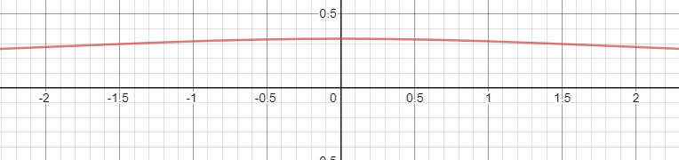
圖 1
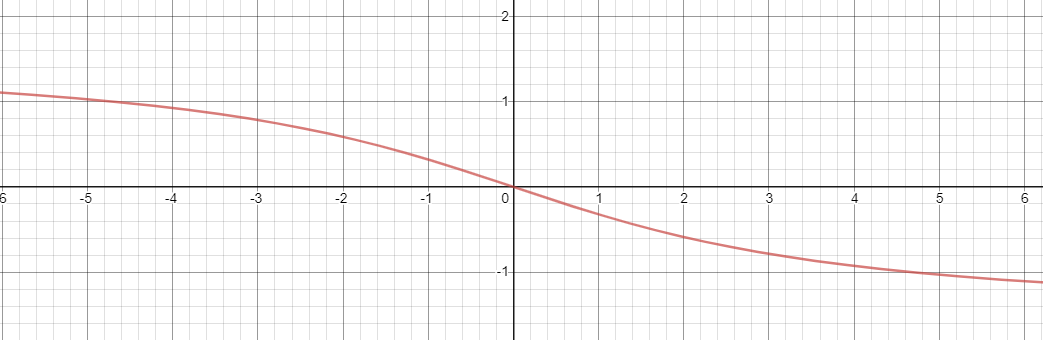
圖 2
Remark:by $\eqref{Fourier6}$
\[X^{*}(\omega)=(\int_{-\infty}^{\infty}x(t) e^{-jk\omega_0 t}dt)^*=\int_{-\infty}^{\infty}x(t) e^{jk\omega_0 t}dt=X(-\omega)\]Examples:
- $x(t)=\delta(t)$, by shifting property
- \[x(t)=\Bigg\{ \begin{aligned} &1 \quad &t \in [-T_1,T_1] \\ &0 \quad &\text{otherwise} \end{aligned}\]
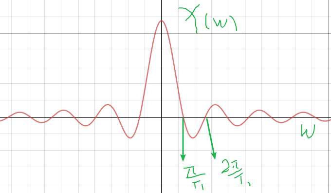
圖 3
Fourier Transform for periodic signals
If $x(t)$ is $T_0$-periodic, then its Fourier transform is
\[X(\omega)=\int_{-\infty}^{\infty}x(t)e^{-j\omega t} dt\]which is not exist in the general cases. However, if we consider Fourier series expression $x(t)$, which is
\[x(t)=\sum_{k=-\infty}^{\infty}X_k e^{jk\omega_0 t}\]and look at the fact that when $x(t)=e^{j\omega_0 t}$, its Fourier transformation $X(\omega)$
\[X(\omega)=\int_{-\infty}^{\infty}e^{j\omega_0 t}e^{-j\omega t} dt =2\pi\delta(\omega_0-\omega)=2\pi\delta(\omega-\omega_0)\]Therefore, it is reasonable to consider
\[\begin{align} X(\omega) &=\int_{-\infty}^{\infty}x(t)e^{-j\omega t}dt \\ &=\int_{-\infty}^{\infty}\sum_{k=-\infty}^{\infty}X_k e^{jk\omega_0 t} e^{-j\omega t} dt \\ &=\sum_{k=-\infty}^{\infty}X_k \int_{-\infty}^{\infty}e^{jk\omega_0 t}e^{-j\omega t} dt \\ &=\sum_{k=-\infty}^{\infty}2\pi X_k\delta(\omega-k\omega_0) \label{FourierSeries_X} \end{align}\]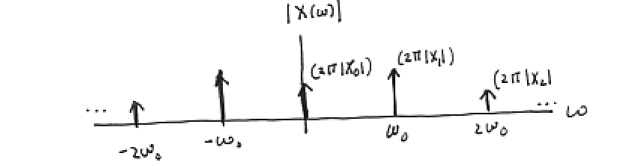
圖 4
Example:
\[x(t)=\sum_{k=-\infty}^{\infty}\delta(t-k)\]We directly compute $X(\omega)$ as following:
\[\begin{aligned} X(\omega)&=\int_{-\infty}^{\infty}\sum_{k=-\infty}^{\infty}\delta(t-k)e^{-j\omega t}dt \\ &=\sum_{k=-\infty}^{\infty}\int_{-\infty}^{\infty}\delta(t-k)e^{-j\omega t}dt \\ &=\sum_{k=-\infty}^{\infty}e^{-j\omega k} \end{aligned}\]Other approaches is to get the Fourier Series Data of $x(t)$. First, observing that $x(t)$ has period $1$, which implies $\omega_0=2\pi$.
According $\eqref{Fourier2}$,
\[\begin{aligned} X_n&=\int_{-1/2}^{1/2} \sum_{k=-\infty}^{\infty} \delta(t-k) e^{-j n \omega t} dt\\ &=\int_{-1/2}^{1/2} \delta(t) e^{-j n \omega t} dt \quad \text{ (since only }\delta(t-0)\text{ has nonzero value in [-1/2,1/2] )} \\ &=\int_{-\infty}^{\infty} \delta(t) e^{-j n \omega t} dt \\ &=e^{-j n \omega 0}=1 \end{aligned}\]Finally, the Fourier seriers data of $x(t)$ is
\[x(t)=\sum_{k=-\infty}^{\infty}e^{-jk2\pi t}\]We have compute the Fourier transform of Fourier series in general, so by $\eqref{FourierSeries_X}$,
\[X(\omega)=\sum_{k=-\infty}^{\infty}2\pi\delta(\omega-k2\pi)\]We prefer the last method one.
Properties of the Fourier Transform
\[\begin{aligned} F(x(t))&=\int_{-\infty}^{\infty}x(t)e^{-j\omega t} dt \\ F^{-1}(X(\omega) )&=\frac{1}{2\pi}\int_{-\infty}^{\infty}X(\omega)e^{j\omega t} d\omega=x(t) \end{aligned}\]- Linearity
- Time Shifting
- Time Scaling If $a\neq 0$
- Differentiation
- Integration
Example: by integration property,
\[F(u(t))=\frac{1}{jw}+\pi\delta(\omega)\]Convolution Property and Frequency Response of LTI Systems
- modulation / frequency shifting
- Convolution
- Freqyency-Domain Convolution
- Inverse Freqyency-Domain Convolution
Example:
\[x(t)=[1+km(t)]cos(\omega_c t)\]where $cos(\omega_c t)$ is called carrier signal, $m(t)$ is called message signal and $k$ is called the modulation index. Assume message singal is banedlimiited by $\omega_m \ll \omega_c$
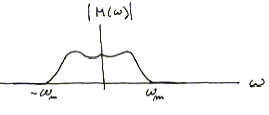
圖 5
We conclude that
\[X(\omega)=\pi(\delta(\omega-\omega_c)+\delta(\omega+\omega_c))+\frac{k}{2} (M(\omega-\omega_c)+M(\omega+\omega_c))\]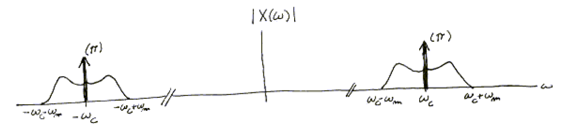
圖 6
Parseval’s Theorem
\[\int_{-\infty}^{\infty} x^2(t)dt=\frac{1}{2\pi}\int_{-\infty}^{\infty}\vert X(\omega)\vert^2 d\omega\]Duality Property
If $x(t)$ has Fourier Transform $X(\omega)$
\[F(X(t))=2\pi x(-\omega)\]Offical 420.214 CT Fourier Transform Table
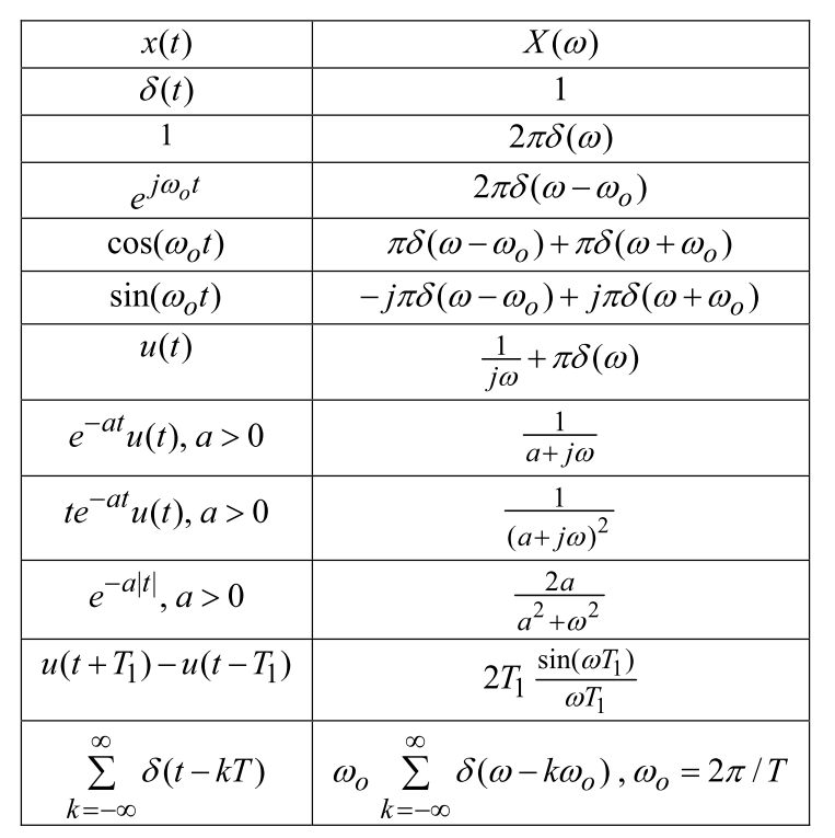
圖 7