
Evaluating
Published:
Evaluating
- Basically, this is my studying from NTCU open course - Machine Learning. I take the key points for my references.
Error rate
\[\text{Error rate }=\frac{\text{Number of misclassified point}}{\text{Total number of data point}}\]k-fold stratified cross validation
Split the data instances into two parts:
- Training set: for learning the classifier
- Testing set: for evaluationg the classifier
Similarly, spliting the data into $k$ equal partitions.
- The labels(+/-) in the training and testing tests should be in right proportion.
- if $k=\text{number or data point}$, this is called nonstratified.
Testing Hypothesis
paired t-test
\[H_0: \bar d=0 \quad v.s. \quad H_1: \bar d\neq 0\]where
\[\bar d=\frac{1}{k}\sum\limits_{i=1}^k d_i, \quad d_i=x_i-y_i\]Here $x_i$ refers the learning method 1 while $y_i$ refers the learning method 2.
\[t=\frac{\bar d}{ \sqrt\frac{\sigma_d^2}{k}}\]$2 \times 2$ confusion matrix
\[C = \begin{bmatrix} \text{True Pos (TP)} & \text{False Neg (FN)}\\ \text{False Pos (FP)} & \text{True Neg (TN)} \end{bmatrix}\] \[\text{Error rate }=\frac{\text{FP}+\text{FN}}{\text{TP+FN+TN+FP}}\]Cost martix
\[C = \begin{bmatrix} 0 & 10(\text{False Neg})\\ 1(\text{False Pos}) & 0 \end{bmatrix}\]Here 10 refers the weight when false negative occurs.
ROC curve
(Receiver Operating Characteristic Curve)
- calculate the probability of being positive class $p(y_i=1)$ for each $i$
- sort order from high to low ($p$)
- draw the ROC curve which the true positive rate as a function of the false positive rate.
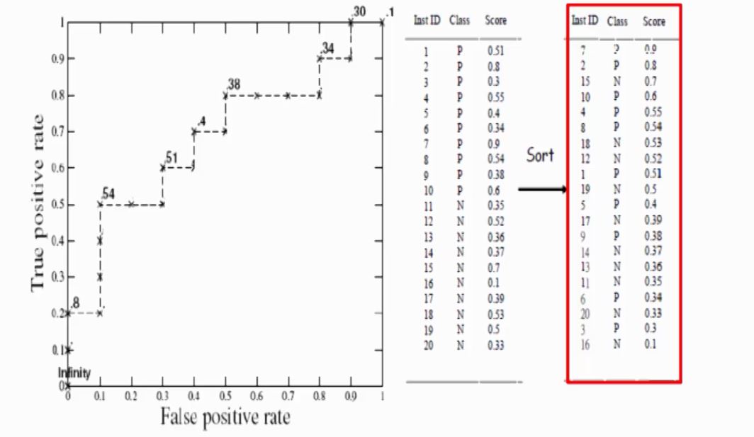
The above two graphs are captured from link.
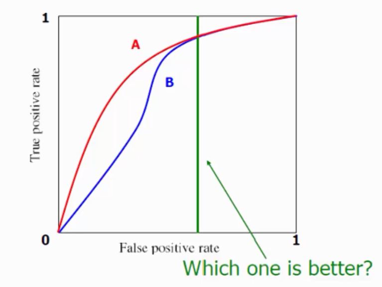
AUC Index
- AUC is an index of ROC curve with range from 0 to 1.
Here,
- $m$: number of positive instances
- $n$: number of negative instances
Recall and Precision
\[\text{Recall}=\frac{\text{TP}}{\text{TP+FN}}\] \[\text{Precision}=\frac{\text{TP}}{\text{TP+FP}}\]Here,
- $\text{FN}$ is relevant but not show as result.
- $\text{FP}$ is irrelevant but as a output.
We are concern Precision more since Recall is difficult to calculate in real cases.
Also, Precision and Recall have reverse relationship.
$\text{precision}=1 \Rightarrow \text{Recall small}$
$\text{Recall}=1 \Rightarrow \text{precision small}$
F-measure
F-meaure balance Recall and Precision
\[F=\frac{2}{\frac{1}{\text{Recall}}+\frac{1}{\text{Precision}}}\]Python code
The following code is retrieved from website
print(__doc__)

import numpy as np
import matplotlib.pyplot as plt
from itertools import cycle

from sklearn import svm, datasets
from sklearn.metrics import roc_curve, auc
from sklearn.model_selection import train_test_split
from sklearn.preprocessing import label_binarize
from sklearn.multiclass import OneVsRestClassifier
from scipy import interp

# Import some data to play with
iris = datasets.load_iris()
X = iris.data
y = iris.target

# Binarize the output
y = label_binarize(y, classes=[0, 1, 2])
n_classes = y.shape[1]

# Add noisy features to make the problem harder
random_state = np.random.RandomState(0)
n_samples, n_features = X.shape
X = np.c_[X, random_state.randn(n_samples, 200 * n_features)]

# shuffle and split training and test sets
X_train, X_test, y_train, y_test = train_test_split(X, y, test_size=.5,
                                                    random_state=0)

# Learn to predict each class against the other
classifier = OneVsRestClassifier(svm.SVC(kernel='linear', probability=True,
                                 random_state=random_state))
y_score = classifier.fit(X_train, y_train).decision_function(X_test)

# Compute ROC curve and ROC area for each class
fpr = dict()
tpr = dict()
roc_auc = dict()
for i in range(n_classes):
    fpr[i], tpr[i], _ = roc_curve(y_test[:, i], y_score[:, i])
    roc_auc[i] = auc(fpr[i], tpr[i])

# Compute micro-average ROC curve and ROC area
fpr["micro"], tpr["micro"], _ = roc_curve(y_test.ravel(), y_score.ravel())
roc_auc["micro"] = auc(fpr["micro"], tpr["micro"])
- plot figure
plt.figure()
lw = 2
plt.plot(fpr[2], tpr[2], color='darkorange',
         lw=lw, label='ROC curve (area = %0.2f)' % roc_auc[2])
plt.plot([0, 1], [0, 1], color='navy', lw=lw, linestyle='--')
plt.xlim([0.0, 1.0])
plt.ylim([0.0, 1.05])
plt.xlabel('False Positive Rate')
plt.ylabel('True Positive Rate')
plt.title('Receiver operating characteristic example')
plt.legend(loc="lower right")
plt.show()